The Kelly Criterion — Does It Work?
This article is originally published at https://quantstrattrader.wordpress.com
This post will be about implementing and investigating the running Kelly Criterion — that is, a constantly adjusted Kelly Criterion that changes as a strategy realizes returns.
For those not familiar with the Kelly Criterion, it’s the idea of adjusting a bet size to maximize a strategy’s long term growth rate. Both https://en.wikipedia.org/wiki/Kelly_criterionWikipedia and Investopedia have entries on the Kelly Criterion. Essentially, it’s about maximizing your long-run expectation of a betting system, by sizing bets higher when the edge is higher, and vice versa.
There are two formulations for the Kelly criterion: the Wikipedia result presents it as mean over sigma squared. The Investopedia definition is P-[(1-P)/winLossRatio], where P is the probability of a winning bet, and the winLossRatio is the average win over the average loss.
In any case, here are the two implementations.
investoPediaKelly <- function(R, kellyFraction = 1, n = 63) {
  signs <- sign(R)
  posSigns <- signs; posSigns[posSigns < 0] <- 0
  negSigns <- signs; negSigns[negSigns > 0] <- 0; negSigns <- negSigns * -1
  probs <- runSum(posSigns, n = n)/(runSum(posSigns, n = n) + runSum(negSigns, n = n))
  posVals <- R; posVals[posVals < 0] <- 0
  negVals <- R; negVals[negVals > 0] <- 0;
  wlRatio <- (runSum(posVals, n = n)/runSum(posSigns, n = n))/(runSum(negVals, n = n)/runSum(negSigns, n = n))
  kellyRatio <- probs - ((1-probs)/wlRatio)
  out <- kellyRatio * kellyFraction
  return(out)
}

wikiKelly <- function(R, kellyFraction = 1, n = 63) {
  return(runMean(R, n = n)/runVar(R, n = n)*kellyFraction)
}
Let’s try this with some data. At this point in time, I’m going to show a non-replicable volatility strategy that I currently trade.

For the record, here are its statistics:
                              Close
Annualized Return         0.8021000
Annualized Std Dev        0.3553000
Annualized Sharpe (Rf=0%) 2.2574000
Worst Drawdown            0.2480087
Calmar Ratio              3.2341613
Now, let’s see what the Wikipedia version does:
badKelly <- out * lag(wikiKelly(out), 2)
charts.PerformanceSummary(badKelly)

The results are simply ridiculous. And here would be why: say you have a mean return of .0005 per day (5 bps/day), and a standard deviation equal to that (that is, a Sharpe ratio of 1). You would have 1/.0005 = 2000. In other words, a leverage of 2000 times. This clearly makes no sense.
The other variant is the more particular Investopedia definition.
invKelly <- out * lag(investKelly(out), 2)
charts.PerformanceSummary(invKelly)

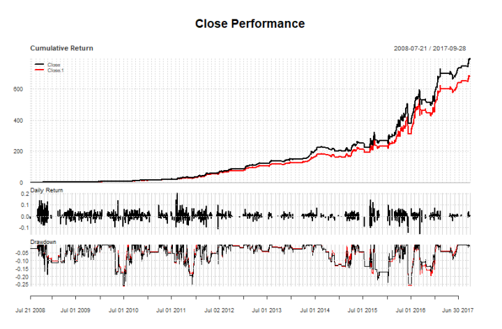
Looks a bit more reasonable. However, how does it stack up against not using it at all?
compare <- na.omit(cbind(out, invKelly))
charts.PerformanceSummary(compare)

Turns out, the fabled Kelly Criterion doesn’t really change things all that much.
For the record, here are the statistical comparisons:
                               Base     Kelly
Annualized Return         0.8021000 0.7859000
Annualized Std Dev        0.3553000 0.3588000
Annualized Sharpe (Rf=0%) 2.2574000 2.1903000
Worst Drawdown            0.2480087 0.2579846
Calmar Ratio              3.2341613 3.0463063
Thanks for reading.
NOTE: I am currently looking for my next full-time opportunity, preferably in New York City or Philadelphia relating to the skills I have demonstrated on this blog. My LinkedIn profile can be found here. If you know of such opportunities, do not hesitate to reach out to me.
Thanks for visiting r-craft.org
This article is originally published at https://quantstrattrader.wordpress.com
Please visit source website for post related comments.
