Sensitivity and Elasticity of seasonal matrix model
This article is originally published at https://tomizonor.wordpress.com
The previous article introduced the seasonal matrices and the population growth rate λ of imaginary annual plant. In this article, let’s try the sensitivity analysis of these matrices and the λ. In sensitivity and elasticity formula, some symbols such as s, v and w are assigned to different meanings from previous.
6. Sensitivity
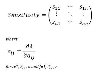
Sensitivity is a partial derivative of λ with respect to each element of transition matrix.
For annual (square) matrix, the sensitivity is calculated as;
![]()
where W denotes right eigenvector, V denotes left eigenvector as an inverse of W, upper * means complex conjugate transpose of matrix, and upper T means transpose of matrix.
sensitivity <- function(A) {
  d <- eigen(A)$values   # eigen values
  w <- eigen(A)$vectors  # right eigen vectors
  v <- Conj(solve(w))    # complex conjugate of left eigen vectors
  # output of eigenvalues is decreasingly sorted.
  v[1,] %*% t(w[,1])
}

> sensitivity(A.spring())
         [,1]      [,2]
[1,] 0.7461573 1.7410337
[2,] 0.1087897 0.2538427

> sensitivity(A.summer())
         [,1]       [,2]
[1,] 0.74615729 15.6693031
[2,] 0.01208775  0.2538427

> sensitivity(A.autumn())
         [,1]       [,2]
[1,] 0.746157290 28.2047456
[2,] 0.006715416  0.2538427

> sensitivity(A.winter())
     [,1]
[1,]    1
For seasonal (non-square) matrices, sensitivities of seasonal elements to annual growth rate are calculated from annual sensitivity matrix calculated above. Because the annual transition matrix starting at winter is a scalar and the value is the λ itself, annual sensitivity at winter must be an identity matrix of size 1 which is given by diag(1), namely, a scalar 1. Knowing this, we can skip the annual sensitivity calculation in this case, because seasonal sensitivities can be calculated by using arbitrary one of four annual sensitivities.
First, let’s try the strict calculation based on annual spring sensitivity.
S1.spring <- function() t(Q()) %*% t(R()) %*% t(S()) %*% sensitivity(A.spring())
S1.summer <- function() t(R()) %*% t(S()) %*% sensitivity(A.spring()) %*% t(P())
S1.autumn <- function() t(S()) %*% sensitivity(A.spring()) %*% t(P()) %*% t(Q())
S1.winter <- function() sensitivity(A.spring()) %*% t(P()) %*% t(Q()) %*% t(R())
Second, do the easy one, based on annual winter sensitivity.
S2.spring <- function() t(Q()) %*% t(R()) %*% diag(1) %*% t(S())
S2.summer <- function() t(R()) %*% diag(1) %*% t(S()) %*% t(P())
S2.autumn <- function() diag(1) %*% t(S()) %*% t(P()) %*% t(Q())
S2.winter <- function() t(P()) %*% t(Q()) %*% t(R()) %*% diag(1)
Both results are identical:
> S1.spring()
       [,1]    [,2]
[1,] 13.5000 31.5000
[2,]  0.2187  0.5103

> S2.spring()
       [,1]    [,2]
[1,] 13.5000 31.5000
[2,]  0.2187  0.5103

> S1.summer()
       [,1]    [,2]
[1,] 2.7000 56.7000
[2,] 0.0243  0.5103

> S2.summer()
       [,1]    [,2]
[1,] 2.7000 56.7000
[2,] 0.0243  0.5103

> S1.autumn()
       [,1]   [,2]
[1,] 0.0135 0.5103

> S2.autumn()
       [,1]   [,2]
[1,] 0.0135 0.5103

> S1.winter()
     [,1]
[1,] 5.000
[2,] 0.729

> S2.winter()
     [,1]
[1,] 5.000
[2,] 0.729
7. Elasticity
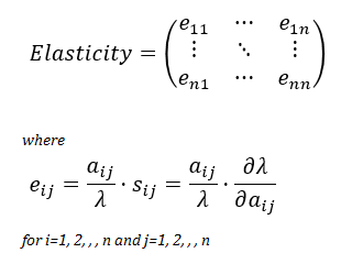
Elasticity is a normalized dimensionless sensitivity as a response to a proportional perturbation.
Elasticity is calculated by

where ○ denotes Hadamard product.
E1.spring <- function() S1.spring() * P() / lambda(A.spring())
E1.summer <- function() S1.summer() * Q() / lambda(A.spring())
E1.autumn <- function() S1.autumn() * R() / lambda(A.spring())
E1.winter <- function() S1.winter() * S() / lambda(A.spring())

> E1.spring()
         [,1]      [,2]
[1,] 0.7461573 0.0000000
[2,] 0.0000000 0.2538427

> E1.summer()
         [,1]      [,2]
[1,] 0.7461573 0.0000000
[2,] 0.0000000 0.2538427

> E1.autumn()
         [,1]      [,2]
[1,] 0.7461573 0.2538427

> E1.winter()
         [,1]
[1,] 0.7461573
[2,] 0.2538427
Because each element of sensitivity matrix differs, comparing sensitivity values across elements can cause misunderstanding. For example, seed production number may have a value of 100 seeds/plant or 10,000 seeds/plant, while survival rate of seedling must be between 0 and 1 as a probability.
We never directly compare these two values; count vs. probability. So we should not directly compare sensitivities of these two elements, too.
Elasticities are safer to compare across elements, because they are normalized to be dimensionless. But still there are pitfalls. Variabilities would differ across elements and across species. So same elasticities doesn’t always mean same importance. Elasticity will be underestimated when a parameter with large variability is near zero by chance.
In the case of this imaginary annual plant, elasticities on the path of spring germination is three-fold greater than that of dormancy seed. Elasticities on the same path are identical, because there’re no differences of importance mathematically between elements on the same path, e.g., plant surviving rate vs. seed production number.
Thanks for visiting r-craft.org
This article is originally published at https://tomizonor.wordpress.com
Please visit source website for post related comments.


