Bayesian model checking via posterior predictive simulations (Bayesian p-values) with the DHARMa package

This article is originally published at https://theoreticalecology.wordpress.com

As I said before, I firmly side with Andrew Gelman (see e.g. here) in that model checking is dangerously neglected in Bayesian practice. The philosophical criticism against “rejecting” models (double-using data etc. etc.) is all well, but when using Bayesian methods in practice, I see few sensible alternatives to residual checks (both guessing a model and stick with it, and fitting a maximally complex model are no workable alternatives imo).

One potential reason for the low popularity of residual checks in Bayesian analysis may be that one has to code them by hand. I therefore wanted to point out that the DHARMa package (disclosure, I’m the author), which essentially creates the equivalent of posterior predictive simulations for a large number of (G)LM(M)s fitted with MLE, can also be used for Bayesian analysis (see also my earlier post about the package). When using the package, the only step required for Bayesian residual analysis is creating the posterior predictive simulations. The rest (calculating the Bayesian p-values, plotting, and tests) is taken care of by DHARMa.

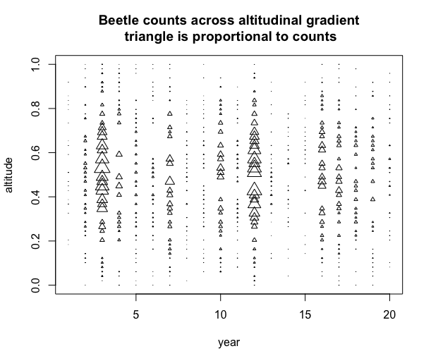
I want to demonstrate the approach with a synthetic dataset of Beetle counts across an altitudinal gradient. Apart from the altitudinal preference of the species (in ecology called the niche), the data was created with a random intercept on year and additional zero-inflation (full code of everything I do at the end of the post).

Now, we might start in JAGS (or another Bayesian software for that matter) with a simple Poisson GLM, testing for counts ~ alt + alt^2, thus specifying a likelihood such as this one

for (i in 1:nobs) {
   lambda[i] <- exp(intercept + alt * altitude[i] +
   alt2 * altitude[i] * altitude[i])
   beetles[i]~dpois(lambda[i])
}

To create posterior predictive simulations, add (and observe) the following chunk to the JAGS model code

for (i in 1:nobs) {
beetlesPred[i]~dpois(lambda[i])
}

The nodes beetlesPred are unconnected, so this will cause JAGS to simulate new observations, based on the current model prediction lambda (i.e. posterior predictive simulations).

We can now convert these simulations into into Bayesian p-values with the createDHARMa function. What this essentially does is to measure where the observed data falls on the distribution of simulated data (see code below, and the DHARMa vignette for more explanations of what that does). The resulting residuals are scaled between 0 and 1, and should be roughly uniformly distributed (the non-asymptotic distribution under H0:(model correct) might not be is not entirely uniform, but in simulations so far, I have not seen a single example where you would go seriously wrong assuming it is). Plotting the calculated residuals, we get:

As explained in the DHARMa vignette , this is how overdispersion looks like. As explained in the Vignette, we should now usually first investigate if there is a model misspecification problem, e.g. by plotting residuals against predictors per group. To speed things up, however, knowing that the issue is both a missing random intercept on year and zero-inflation, I have created a model that corrects for both issues.

So, here’s the residual check with the corrected (true model) – now, things looks fine.

When doing this in practice, I highly recommend to not only rely on the overview plots I used here, but also check

1. Residuals against all predictors (use plotResiduals with myDHARMaObject$scaledResiduals)
2. All previous plots split up across all grouping factors (e.g. plot, year)
3. Spatial / temporal autocorrelation

which is all supported by DHARMa.

There is one additional subtlety, which is the question of how to create the posterior predictive simulations for multi-level models. In the example below, I create the simulations conditional on the fitted random effects and the fitted zero-inflation terms. Most textbook examples of posterior predictive simulations I have seen use this approach. There is nothing wrong with this, but one has to be aware that this doesn’t check the full model, but only the final random level, i.e. the Poisson part. The default for the MLE GLMMs in DHARMa is to re-simulate all random effects. I plan to discuss the difference between the two options in more detail in an extra post, but for the moment, let me say that, as a default, I recommend re-simulating the entire model also in a Bayesian analysis. An example for this extended simulations is here.

The full code for the simple (conditional posterior predictive simulation) example is here

Thanks for visiting r-craft.org
This article is originally published at https://theoreticalecology.wordpress.com
Please visit source website for post related comments.